YP Paper reading / 2026
Get the paper ↓

PNAS · 2026 WANG & DOKHOLYAN OPEN ACCESS

AlphaFold hands you the protein.
It does not tell you where the drug goes.

Structure prediction is close to solved. Finding the pocket on that structure is not. It is a separate problem, it sits upstream of every docking run and every screen, and getting it wrong cannot be recovered downstream. YuelPocket's answer is one extra node in the graph.

Protein residues and ligand atoms connected through a single virtual joint node Red nodes on the left are protein residues, blue nodes on the right are ligand atoms. Rather than connecting every residue to every atom, both sides connect to one white node in the middle. JOINT
protein residues ligand atoms one virtual node
309,140training systems, from PLINDER
m + nedges instead of m × n
62%Top-1 pocket centre within 4 Å, against 55% for P2Rank
15probe molecules cover most pockets
01

THE QUESTION

The introduction, unpacked

A structure is not a target.

Two hundred million protein structures are now a database lookup. That changed what the hard part is. If you want to drug a protein you still have to answer a question the structure does not contain: out of a surface with thousands of atoms, which patch actually binds a small molecule, and which small molecule.

This paper is unusually direct about why that matters. Its significance statement argues that failures in virtual screening and lead optimisation are often caused by identifying the wrong site in the first place, rather than by any weakness in the docking algorithm or the scoring function that runs afterwards. That is a claim about where in the pipeline the error lives, and it is worth taking seriously, because errors at the front of a pipeline do not average out. They propagate.

Why the first step is the expensive one

Everything after the pocket assumes the pocket.

Docking searches poses inside a box you give it. Scoring ranks what docking found. Screening ranks what scoring scored. None of those stages can tell you that the box was in the wrong place. They will return a confident, well-ranked, entirely useless answer.

  1. 01Binding sitewhich patch of surface
  2. 02Dockingposes inside that box
  3. 03Scoringrank the poses
  4. 04Virtual screenrank the library
  5. 05Lead optimisationchemistry, months of it
$2.6Bdevelopment cost per approved drug
~90%of candidates fail in clinical trials
0of that is recovered by a better scoring function if the site is wrong

But AlphaFold 3 places ligands now

It does. Just not reliably enough to build on.

AlphaFold 3 predicts protein and small molecule together, which looks like it should retire this whole problem. The paper cites an assessment by Shen and colleagues finding that while the receptor structure comes out reliably, the position of the small molecule is variable and frequently inaccurate. The gap is widest exactly where it hurts most: allosteric modulators, the sites you go looking for when the orthosteric pocket is undruggable.

So the two problems separate again. Predicting the fold and predicting the functional site are not the same task, and solving the first did not solve the second.

SOLVED The fold

Receptor backbone comes out reliably

NOT SOLVED The site

Ligand placement variable, worst on allosteric modulators

Schematic. The bars stand for the qualitative gap the paper describes, not measured values.

What came before

Three generations of pocket finders,
and the blind spot each one kept.

Select a generation to see how it looks at a protein, and where that view runs out.

FOUND MISSED FIXED BOX OUT OF RANGE LOCAL RADIUS NOT CONNECTED

The other half of the problem

How much data each method learned from.

02

THE MOVE

One node, added on purpose

Connect everything to one thing
instead of everything to each other.

The obvious way to let a protein and a ligand talk to each other in a graph is to connect every residue to every atom. It works, and it is unusable: with m residues and n atoms you have written down m × n edges, and that number grows faster than any real protein lets you afford.

YuelPocket puts a single virtual node between the two sides. Every residue connects to it, every ligand atom connects to it, and nothing connects directly across. Information still flows both ways, in two hops instead of one, and the edge count collapses from m × n to m + n.

The whole argument, in one slider

Drag a real protein into the graph.

Both designs carry the same structural edges: backbone links, residue contacts, chemical bonds. That shared count is written as C in the paper. What differs is how the two sides are joined.

All-to-all 0 C + m × n
Virtual joint node 0 C + m + n

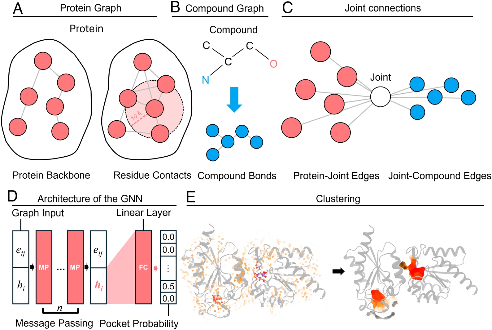
PAPER FIGURE 1Graph construction and network
Five panels: a protein graph of alpha carbon nodes with backbone and contact edges, a compound graph of heavy atoms and bonds, the joint connection topology through a virtual node, the message passing network, and a clustering visualisation.

The whole design on one page. Panels A and B are the two molecules as graphs; panel C is the entire contribution of the paper.

A
Protein graph. Red nodes sit on alpha carbons, edges are backbone links and residue contacts inside 8 Å.
B
Compound graph. Blue nodes are heavy atoms, edges are chemical bonds.
C
The joint connection. Both sides attach to one white virtual node rather than to each other, which is what turns m × n edges into m + n.
D
The network. Sixteen rounds of message passing with learned edge weights, then a linear head returning a pocket probability per residue.
E
Clustering. Scored surface points collapsed into discrete pocket locations.

Reproduced from Wang & Dokholyan, PNAS 2026, figure 1, under CC BY 4.0.

REPRESENTATION

Two nodes per residue

Each residue becomes a backbone node at the alpha carbon and a side-chain node at the geometric centre of its side chain, in the spirit of the UNRES coarse-grained force field. Coarse enough to stay robust to small errors, detailed enough to keep side-chain geometry in play.

FEATURES

Five numbers on every edge

Each edge carries the Euclidean distance plus four binary flags: is this a protein contact, a chemical bond, a protein-to-virtual link, or a ligand-to-virtual link. Nodes carry a one-hot identity and a three-way mask marking them protein, ligand or virtual.

TRAINING

Two heads, two losses

One head asks whether this protein and this ligand belong together at all, trained contrastively against 50 decoy ligands. The other predicts per-residue pocket probability from the element-wise product of the residue embedding and the ligand's virtual node. Dice loss switches on only once the F1 score passes 0.2, so it refines rather than destabilises.

03

TWO MODES

Two different questions, two different answers

Which residues,
and where exactly.

These are not the same output, and the paper is right to separate them. A list of contact residues tells you about mechanism. A set of coordinates tells docking where to put its box. YuelPocket runs both from the same trained network.

Solvent accessible surface probes over protein 7T8F, coloured by predicted score. The same probes after hill-climbing clustering, collapsed into two ranked pocket centres.
THE PART THAT IS EASY TO SKIM PAST

How a probability becomes a coordinate.

The coordinate mode reformulates pocket finding as a ranking problem. Shrake-Rupley rolls a 1.4 Å solvent probe over the protein and every surviving surface point becomes a candidate pocket centre. Each candidate gets its own small graph: nearby residues within 10 Å, all ligand atoms, and the probe itself acting as a local hub, exactly like the virtual joint node does globally.

Then those raw scores have to become discrete sites. Each surface point climbs toward its highest-scoring neighbour, points that converge on the same peak get merged with a union-find structure, and the peaks become ranked pocket centres. It is a small piece of engineering, and it is what turns a cloud of numbers into something a docking program can accept.

04

THE EVIDENCE

Tested where it is hard to cheat

PLINDER splits on three axes at once.

Training and test are separated by 30% protein sequence similarity, 30% protein-ligand interaction similarity and 50% ligand Tanimoto similarity, all at the same time. 309,140 systems for training, 832 for validation, 1,036 held out. The authors also dropped COACH420 entirely after finding most of it already sat inside PLINDER's training data, which is the kind of decision that costs you a favourable number and buys you a trustworthy one.

Residue level

"Correct" here is a ranking, not a yes or no.

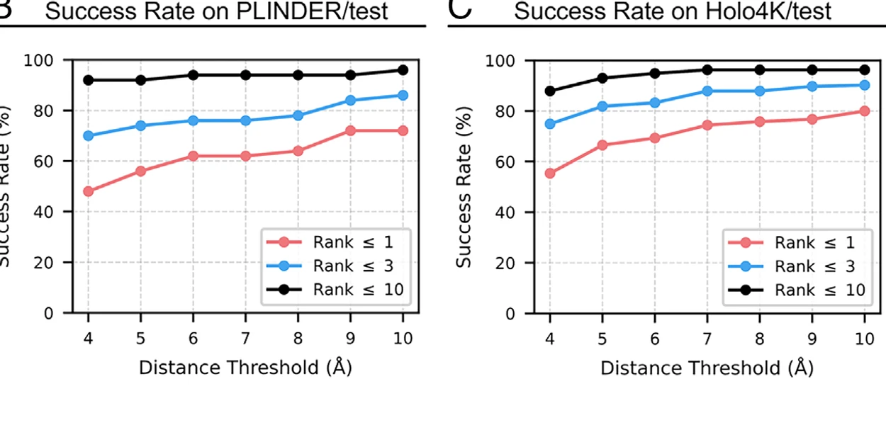
The model returns a probability for every residue, so success has to be defined against two dials: how many guesses you allow, and how close counts as close. A prediction succeeds if at least one of the top K residues lands within D ångström of any ligand atom.

Which dial setting is the real number depends on what you are doing. Top-1 at 4 Å is what to quote if you get one shot at the site. Top-10 at 8 Å is what matters if you intend to dock into everything plausible and let scoring sort it out afterwards.

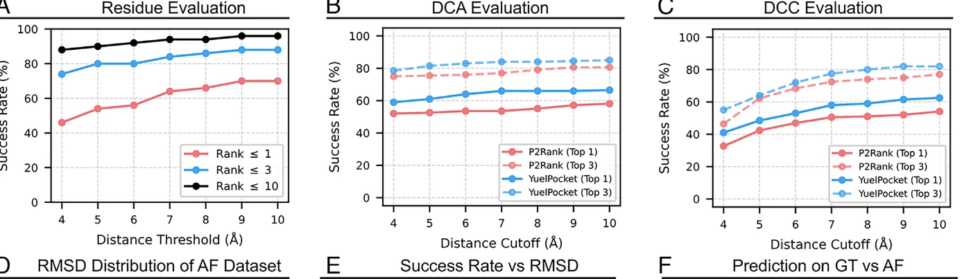
Two line charts of success rate against distance threshold, one for PLINDER and one for Holo4k, each with curves for rank within 1, 3 and 10.
Figure 2B, 2C. PLINDER on the left, Holo4k on the right. Red is Top-1, blue Top-3, black Top-10. Top-1 at 4 Å starts near 48% on PLINDER and reaches roughly 70% by 10 Å. The black curve sits above 90% almost everywhere, which is the useful message: the site is nearly always somewhere in the top ten even when the single best guess misses.

What the output actually looks like

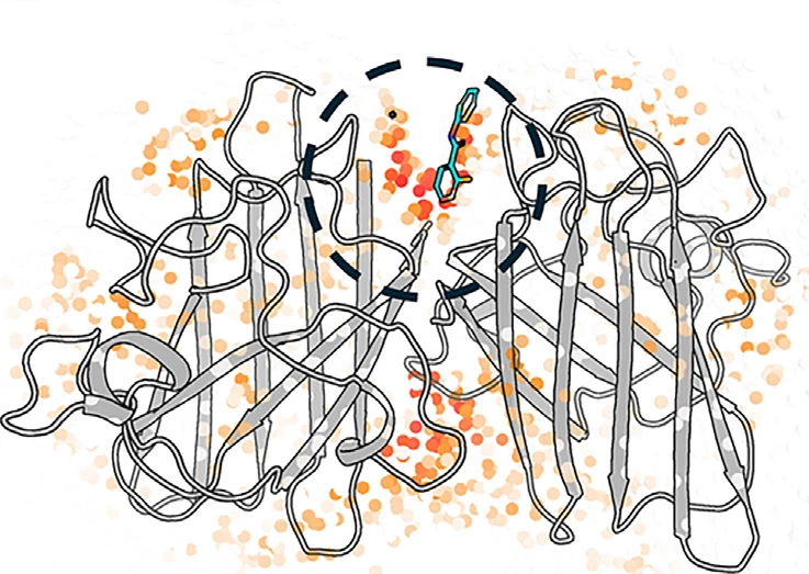
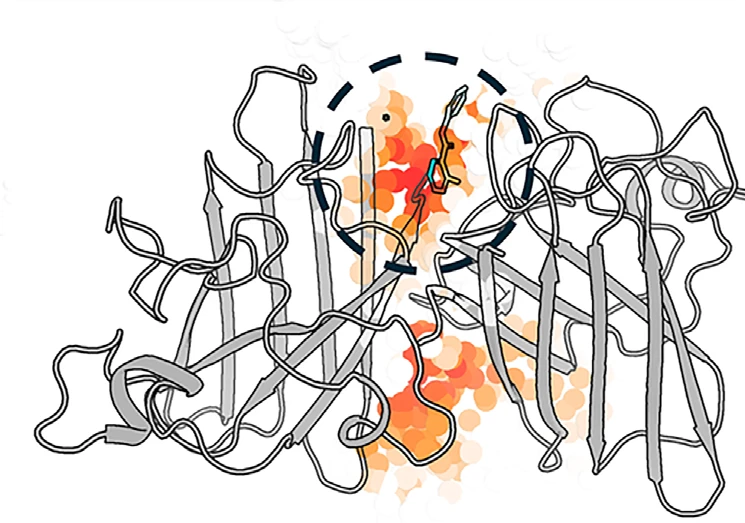
Including at the seam between two subunits.

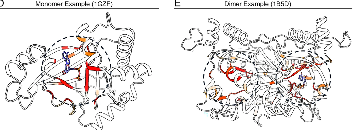
Curves say how often it works. A coloured structure says what "working" looks like, and the second of these two is doing more than decoration. A large share of real binding sites form at the interface between subunits, where the pocket is made of residues contributed by two different chains.

That is the exact case a local graph handles worst, because the two halves of the site may be far apart along every path the graph knows about. Showing a dimer here is the paper quietly answering the objection it raised in its own introduction.

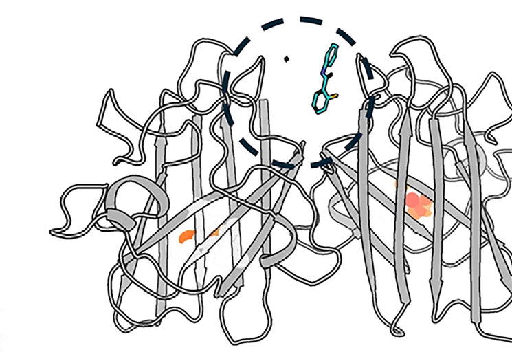
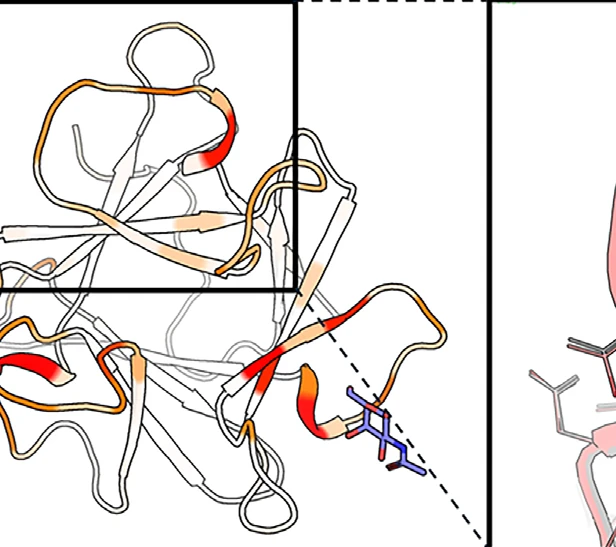
Two protein cartoons coloured by predicted pocket probability, a monomer and a dimer, with the predicted sites circled.
Figure 2D, 2E. Monomer 1GZF on the left, dimer 1B5D on the right, both coloured by predicted probability from white through orange to red. Dashed circles mark the true sites.

Two ways to be right

Did you find the pocket,
or did you find its middle?

Coordinate predictions get scored with two different distances, and the difference matters more than it sounds. Distance to Closest Atom measures from the predicted centre to the nearest atom of the real ligand: it asks whether you landed on the site at all. Distance Centre-to-Centre measures to the ligand's centroid: it asks whether you also read the shape of the site correctly.

The second is strictly harder and the gap shows it. You can be inside the right pocket and still put its centre in the wrong place, which is precisely the error that sends a docking box off target.

ligand centroid predicted centre DCA · centre to nearest ligand atom DCC · centre to ligand centroid Drawn for this page · schematic

Against the standard baseline

The lead is real on PLINDER.

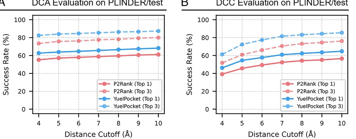
P2Rank is the sensible thing to measure against: widely used, template free, fast. On the hard split YuelPocket is ahead on both distance measures, by roughly seven points at Top-1 within 4 Å on the first and five on the second.

Note how much lower every DCC curve sits than its DCA counterpart. That gap is the same one the diagram above describes, and it is a property of the task rather than of either method.

Two line charts on the PLINDER test set, distance to closest atom and distance centre to centre, comparing YuelPocket in blue against P2Rank in red at Top-1 and Top-3.
Figure 3A, 3B. PLINDER test set. Blue is YuelPocket, red is P2Rank; solid lines are Top-1, dashed are Top-3. Left is distance to the closest ligand atom, right is centre to centre.

And on the easier one

On Holo4k the two methods nearly meet.

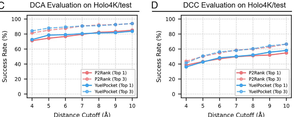
This is the panel a less careful paper would have left out. On Holo4k the curves converge and the advantage mostly disappears, and rather than bury that, the discussion explains it: PLINDER's construction discards a large slice of the archive on similarity grounds, so the Holo4k systems that survive filtering are likely drawn from that discarded pool and sit closer to training data.

Read together, the pair says something more useful than either alone. The harder the split, the bigger the gap, which is the shape you want if the claim is about generalisation rather than fit.

The same two distance measures evaluated on the Holo4k test set, where the YuelPocket and P2Rank curves nearly coincide.
Figure 3C, 3D. Holo4k, same two measures and the same colour scheme. The lead narrows to almost nothing here, which section 06 returns to.

The same protein, two methods

7T8F, scored and then clustered.

Curves aggregate away the thing you most want to see, which is what a good and a bad prediction look like side by side. Step through the four states: raw surface scores first, then what survives clustering, for each method in turn. The dashed circle marks the true site.

YuelPocket produces a dense, confident cloud that collapses onto the right place. P2Rank's scores on this system are sparse enough that the clustered centre drifts off the ligand entirely.

7T8F scored by YuelPocket, dense orange probe cloud concentrated near the true site. 7T8F after clustering YuelPocket scores, top two clusters at the true site. 7T8F scored by P2Rank, sparse scattered points. 7T8F after clustering P2Rank scores, clusters away from the true site.

The test that actually matters now

Nobody is going to hand you
a crystal structure.

The reason this is useful in 2026 is that most targets arrive as predicted structures. So the authors ran AlphaFold on all 1,036 PLINDER test proteins and evaluated on those instead of on the experimental ones.

Performance holds

And the margin gets wider, not narrower.

Top-3 residue success stays above 70% at 4 Å and Top-10 above 90%. The interesting part is the coordinate comparison: the lead over P2Rank grows to roughly ten percentage points on predicted structures, larger than on experimental ones.

That direction makes sense given the design. A coarse-grained representation that deliberately ignores fine atomic detail should degrade more gently when the atomic detail is itself a prediction.

Three charts of success on AlphaFold predicted structures: residue level by rank, and coordinate level by both distance measures against P2Rank.
Figure 4A, 4B, 4C. All evaluated on AlphaFold models rather than crystal structures. Residue level on the left; the two coordinate measures on the right, blue YuelPocket against red P2Rank.

Where the errors come from

Side chains, not folds.

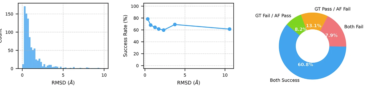
The middle panel is the one worth pausing on. Success dips as the predicted structure drifts from the crystal, then stops falling and flattens, which is not what you would expect if bad folds were driving failure.

The authors' reading: at low deviation the damage is side-chain placement, which the model is partly sensitive to despite the coarse representation. At high deviation the error is usually how subunits sit relative to each other in an oligomer, while the individual monomers, and therefore their pockets, are still fine.

A histogram of backbone deviation for the AlphaFold models, a plot of success rate against that deviation, and a donut chart of agreement between experimental and predicted runs.
Figure 4D, 4E, 4F. How far the models sit from experiment, success against that distance, and the agreement between the two runs. About 61% succeed on both; roughly 13% work on the crystal but fail on the prediction. The four slices printed in the donut sum to 90%, so one of its labels appears to be mistyped. The numbers quoted here come from the paper's text instead.

One case, both ways

4I4V, solved and predicted.

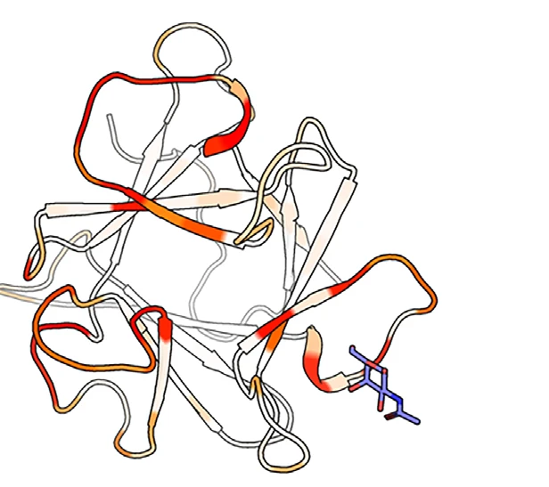
The same pocket is identified on the experimental structure and on the AlphaFold model. Subtle side-chain rotations between the two shift the predicted probabilities slightly without moving the site, which is the concrete version of the trend in the panels above.

Protein 4I4V experimental structure coloured by predicted pocket probability. The AlphaFold model of 4I4V, with the same pocket identified.

Figure 4G and 4H · PDB 4I4V

05

PROBES

A consequence the authors turned into a method

If the answer depends on the ligand,
ask with the right ligand.

Because YuelPocket conditions on a specific molecule, the same protein returns different pockets for different inputs. That could be filed as an inconvenience. Instead the paper turns it into a tool: pick a small set of molecules that between them light up as many distinct sites as possible, and use them as probes.

How the set is built

Greedy, and it converges fast.

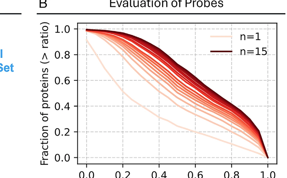
Start with nothing. Each round, score every candidate ligand by how many previously uncovered pocket residues it would newly reach across a batch of proteins, add the winner, repeat until coverage passes threshold. No learning, no optimisation, just a coverage argument.

Fifteen molecules is where it stops being worth adding more. The curves show the return diminishing steadily rather than cliff-edging, which suggests the set could be trimmed or extended depending on how much compute you want to spend per target.

A family of curves showing the fraction of proteins exceeding a recall threshold, one curve per probe set size from one to fifteen.
Figure 5B. Each curve is one more probe in the set, palest for a single probe and darkest for all fifteen. The x-axis is how much of a protein's true pocket you demand; the y-axis is the fraction of proteins clearing that bar. The whole family lifts as the set grows.

What got chosen

Three unremarkable molecules.

This is the part worth staring at. The top three probes are not designed, not privileged, not chemically exotic. They are ordinary ligands lifted out of ordinary structures, and their value is purely that their pocket predictions happen to be complementary to each other.

Which tells you the property being exploited is not about the molecules at all. It is about what the network has learned to key on when it conditions a prediction, and a probe is just a handle for steering that.

Chemical structures of the three top ranked probe molecules, KI2, PTY and FER.
Figure 5C. KI2 from PDB 1NH0, PTY from 3AR4, FER from 3CBG. Ranked by how much new pocket coverage each one contributed.

1D1V, asked twice

The native ligand only finds its own pocket.

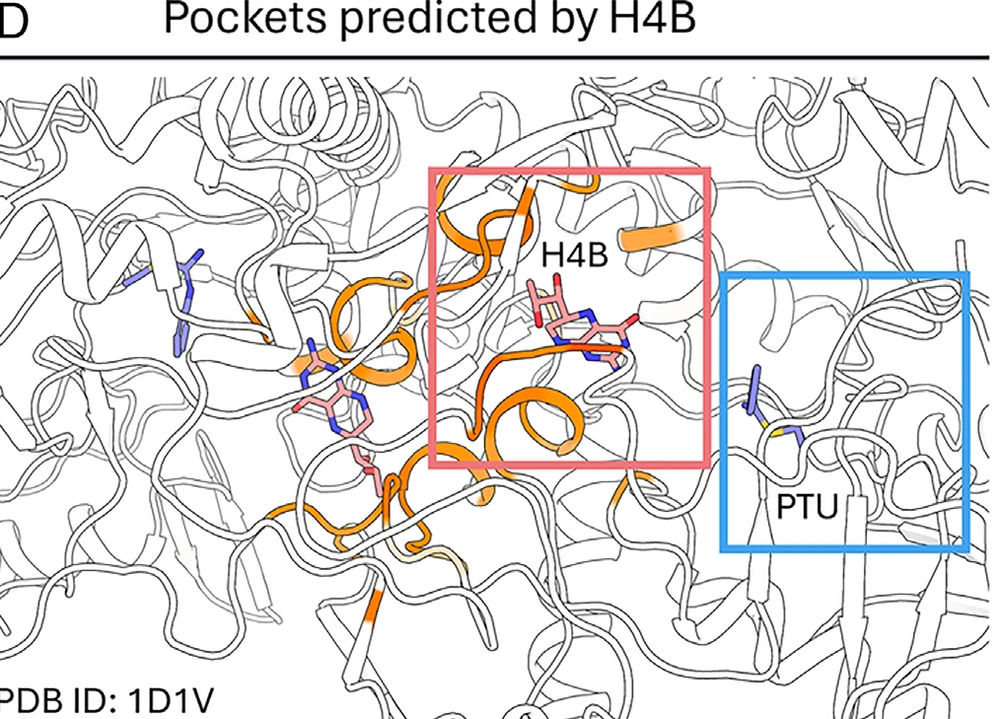
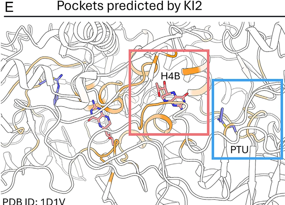
Query this protein with H4B, the ligand it actually crystallised with, and the model confidently marks the H4B site and essentially ignores the PTU site. Query it with KI2 from the probe set instead, and both light up. The H4B site loses a little confidence in exchange, which the authors accept as a fair trade for finding a pocket you would otherwise never have looked at.

Protein 1D1V queried with H4B. The H4B box is coloured, the PTU box is not. Protein 1D1V queried with probe KI2. Both the H4B and PTU boxes carry signal.
06

THE EDGES

Read the discussion, not just the abstract

Where this stops.

The paper is unusually willing to explain away its own good numbers. That is worth more than the numbers.

01

The easier benchmark is easier, and they say so

Holo4k scores higher than PLINDER throughout. Rather than lead with the better figure, the authors explain it: PLINDER's construction throws out a large fraction of the archive on similarity grounds, so the 300 Holo4k-only complexes are likely drawn from that discarded pool and sit closer to training data. PLINDER is the lower bound and should be read as the real one.

02

Coarse-grained cuts both ways

Two nodes per residue buys robustness to imperfect structures. It also throws away atomic detail that sometimes decides which residues line a pocket. The authors note that dropping to backbone alone would simplify the model further and would probably cost accuracy, and leave the trade open.

03

Top-1 at 4 Å is still under half

48% on PLINDER. The headline numbers are Top-3 and Top-10, and those are legitimate for a workflow where you dock into several candidate sites. They are not the same as getting it right first time, and a reader skimming the abstract could easily come away thinking they are.

04

Shallow sites report low confidence

The 1DY4 example in the supplement shows the same protein returning quite different maps for different query ligands, with shallow sites producing weak signal. That is arguably correct behaviour, since shallow sites do bind more weakly. It also means a low score is ambiguous between "not a pocket" and "a poor pocket".

05

You have to bring a molecule

Conditioning on the ligand is the source of most of what is interesting here, and it is also a requirement. For a fresh target with no known binder you are choosing probes rather than reading off an answer, and the fifteen-probe set is a starting point rather than a guarantee of coverage.

THE SHORT VERSION

The contribution is not a bigger network.
It is a cheaper way to let two molecules talk.

One virtual nodeGlobal reach, linear costCondition on the ligandDifferent molecule, different pocket

Strip away the benchmarks and the argument is small and structural. Everyone agreed graphs were the right representation for a protein and a ligand together. The blocker was that joining them properly costs m × n edges, so the field built local graphs instead and quietly gave up on long-range cooperation. Routing both sides through a single node makes the global graph affordable, and once it is affordable the model can be trained on three hundred thousand systems rather than a few thousand. The binding affinity correlation nobody asked for is the sign that the representation learned something real.

READ IT YOURSELF

The paper,
in full.

Published open access under a Creative Commons Attribution 4.0 licence, which is also why every figure on this page can be shown here with attribution. Mirrored locally so the download works regardless of what PNAS is doing.

COLOPHON

An interactive reading of Wang & Dokholyan, PNAS 2026. All numbered figures are reproduced from the paper under its CC BY 4.0 licence. Diagrams in the opening section are drawn for this page and are schematic, not reproductions. The work was supported by the National Institutes of Health (1R35 GM134864, R01 AT012053, R01 AG071675) and the National Science Foundation (2210963).