YD Paper reading / 2026
Get the paper ↓

SCIENCE ADVANCES · 2026 WANG, ZHANG, BUDAKOTI, DOKHOLYAN CC BY 4.0

Every molecule designer before this one
nailed the pocket shut.

Proteins change shape when something binds to them. Diffusion models that design drugs into pockets have almost all treated the pocket as a fixed wall, because letting it move means generating the protein and the ligand at once. YuelDesign generates both, and the consequence is not a better score. It is a class of molecule that was previously impossible to design.

A pocket opening to admit a ligand A protein pocket drawn as a ring of side chains. Two of them are bridged to each other, closing the entrance. When the bridge breaks the side chains swing apart and a ligand seats inside. SALT BRIDGE — CLOSED

~400atoms generated at once, against 15–50 for ligand-only methods
1.8 Åmedian deviation of the generated pocket from the real one
2.84 Åthe salt bridge distance it has to be able to break
2diffusion processes running on one object
01

THE QUESTION

The introduction, unpacked

A pocket is not a hole.

Structure-based drug design starts by pointing at a cavity on a protein and asking a model to fill it. The convenient assumption is that the cavity is a fixed shape you design against, like fitting a key to a lock. Biology has known for sixty years that this is wrong, and has a name for why.

Koshland's induced fit says the pocket and the ligand shape each other on contact. Side chains rotate, contacts break and reform, and the cavity that finally holds the drug is not the cavity you started from. Docking software has taken this seriously for a long time: flexible docking exists precisely because rigid docking gets binding modes wrong.

Generative models mostly did not follow. The reason is not carelessness — it is that letting the pocket move means generating the protein too, and that changes the size of the problem.

What the field had built

Two branches, and one assumption they share.

Molecular generation split early. One branch writes molecules as text or graphs and never touches 3D at all. The other places atoms in space, conditioned on a pocket. Only the second branch can design into a specific target, which is why structure-based work lives there.

Select a branch to see what it generates, and what it assumes about the protein.

MOLECULE ONLY CC(=O)Nc1ccc(O)cc1 no protein anywhere in the model MOLECULE IN A FIXED POCKET FIXED pocket is a boundary condition, never an output MOLECULE AND POCKET TOGETHER both are outputs of the same denoising process

Why nobody did this sooner

Letting the pocket move multiplies what you generate.

Ligand alone
15–50 atoms
Ligand + pocket, all atom
up to ~400 atoms

Diffusion works on every atom simultaneously, so the dimensionality of the object being denoised is what grows. That is not a constant-factor problem: the paper is explicit that generation quality falls off for larger molecules for exactly this reason, and suggests latent diffusion as the way out. Roughly an order of magnitude more atoms is the price of admission for a pocket that moves, and it is why the rigid assumption survived as long as it did.

02

THE MOVE

Generate both, from one noise draw

The pocket stops being
a boundary condition.

YuelDesign puts the pocket atoms and the ligand atoms into a single coordinate matrix, keeps track of which is which with binary masks, and denoises the whole thing. Nothing in the architecture privileges the protein as fixed scenery. Side chains rearrange as the ligand forms, because both are being predicted by the same network at the same timestep.

Training data is Binding MOAD, about 41,409 structures with measured affinities for 15,223 of them. The binding site is defined as every residue with an atom within 6 Å of the ligand. The split is filtered on three axes at once — sequence identity above 30%, pocket deviation below 2 Å, or ligand Tanimoto above 0.85 all force a pair into the same side of the split — so near-duplicates cannot straddle train and test.

The loop, end to end

Extract, destroy, rebuild, then infer the bonds.

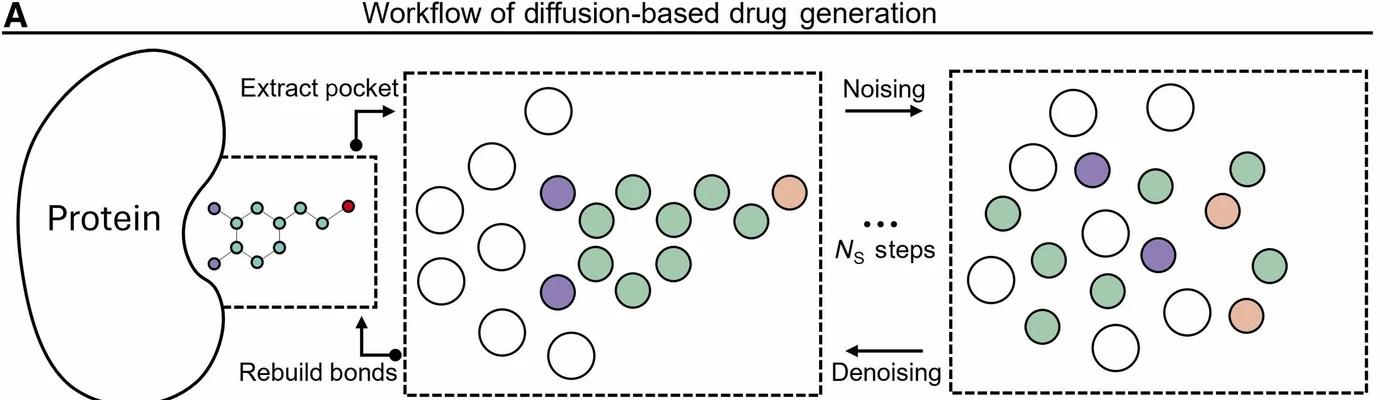
Cut the pocket out of the protein, add noise to the whole assembly over a fixed number of steps until nothing is left, then run the reverse process to bring back a pocket and a molecule together.

The last step is worth noticing: bonds are reconstructed after denoising, from the interatomic distances that came out. The model never generates a bond. This is why connectivity is a metric to be measured rather than a property that is guaranteed, and why fragmented molecules are a real failure mode for every method in this family.

Workflow diagram: a pocket is extracted from a protein, noise is added over N steps until the atoms are unstructured, denoising reverses the process, and bonds are rebuilt at the end.
Figure 1A. The generation loop. White circles are pocket atoms, coloured circles are ligand atoms — both are inside the noising box, which is the entire point. Reproduced from Wang et al., Science Advances 2026, under CC BY 4.0.

What one denoising step sees

Three representations, one network.

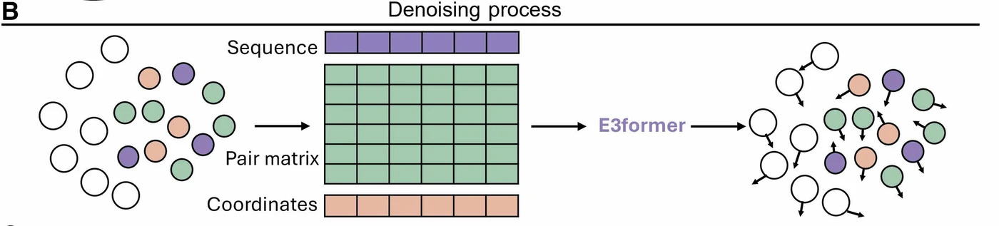
Atom identities become a sequence of features. Every atom pair becomes an entry in a matrix. The coordinates ride alongside as their own track. E3former consumes all three and returns displacements, drawn here as arrows on each atom.

Because the pair matrix is over every atom in the assembly, a pocket side chain and a ligand atom are entries in the same matrix. Neither has any special status.

A denoising step: a cloud of atoms becomes sequence features, a pair matrix and coordinates, which pass through E3former and come back as per-atom displacement arrows.
Figure 1B. Sequence in purple, pair matrix in green, coordinates in orange. The arrows on the right are the predicted displacements for this step. Reproduced from Wang et al., Science Advances 2026, under CC BY 4.0.

One object, two kinds of noise

Coordinates are continuous. Atom identity is not.

A carbon does not become an oxygen by sliding gradually through intermediate elements. So the two things being generated need different noise processes, and YuelDesign runs both at once: an elucidated diffusion model over positions, and a discrete denoising diffusion model over atom types, sharing the same network features and the same timestep.

Sharing matters. Because both read the same representation, the model can learn that a particular local geometry wants a particular element there, rather than deciding shape and chemistry independently and hoping they agree.

CONTINUOUS · positions EDM · Gaussian noise on coordinates
DISCRETE · identities D3PM · categorical jumps between elements
03

THE MACHINE

Where the architecture came from

An Evoformer that outputs coordinates.

The backbone is called E3former, and it is AlphaFold's Evoformer stack adapted for a job Evoformer was not built to do. Evoformer reasons over sequence and pair features and emits a distogram — a prediction about distances. E3former keeps the triangular attention and multiplication that make that reasoning work, then ends in an equivariant coordinate head that emits atomic displacements directly.

WHAT WAS REMOVED

No alignments, no positions

Evoformer consumes multiple sequence alignments and positional encodings. Neither survives here, and for a good reason: a pocket carved out of a protein plus a small molecule has no canonical ordering to encode, and no meaningful alignment. E3former runs single-sequence attention over an unordered bag of atoms.
WHAT WAS ADDED

An equivariant coordinate head

The final pair embeddings are turned into displacements by aggregating weighted direction vectors between atoms. Because every update is built from vectors between atoms rather than from absolute positions, rotating or translating the input rotates or translates the output identically, and the model never has to spend capacity learning that physics is orientation independent.

WHAT IT COSTS

Triangles over 400 atoms

Triangle attention is what lets distant atoms constrain each other, and it is also why the atom count matters so much. The paper does not report a compute budget, but the limitation it does report — degradation on larger molecules — points at this being the binding constraint.

The block that does the work

Triangles, then a coordinate head.

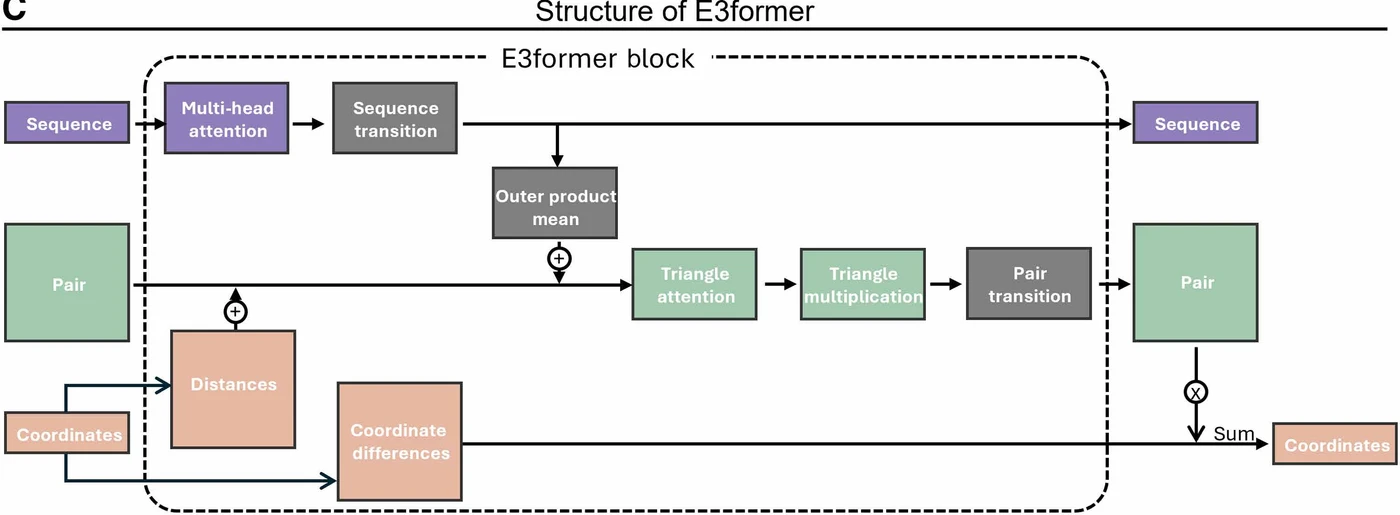
Sequence features carry what each atom is. Pair features carry how every atom relates to every other. Triangle attention and triangle multiplication are the operations that let three-way consistency propagate — if atom i relates to j, and j to k, then the i-to-k relationship is constrained too, which is how geometry stays coherent over a molecule the network never sees as a whole.

Everything to the left of the dashed box is inherited from Evoformer. Everything in the bottom row is not: distances and coordinate differences feed in, and the block ends by summing weighted direction vectors into a coordinate update.

Block diagram of an E3former block: sequence features pass through multi-head attention and a transition, pair features through triangle attention, triangle multiplication and a pair transition, and coordinates enter as distances and coordinate differences before a weighted sum produces updated coordinates.
Figure 1C. One E3former block. Purple is sequence, green is pair, orange is coordinates. The dashed outline is the repeated block. Note that coordinates enter only as distances and differences between atoms, never as absolute positions, which is what makes the output rotate and translate with the input. Reproduced from Wang et al., Science Advances 2026, under CC BY 4.0.
04

THE EVIDENCE

First, does it produce real molecules

Before flexibility can matter,
the chemistry has to be sane.

Diffusion models place atoms independently and infer bonds afterwards, which means a generated molecule can come out in disconnected pieces or wrapped in strained rings that no chemist would make. These are not aesthetic complaints; they decide whether the output is a molecule at all.

Against two rigid-pocket baselines

Connectivity holds as molecules get bigger.

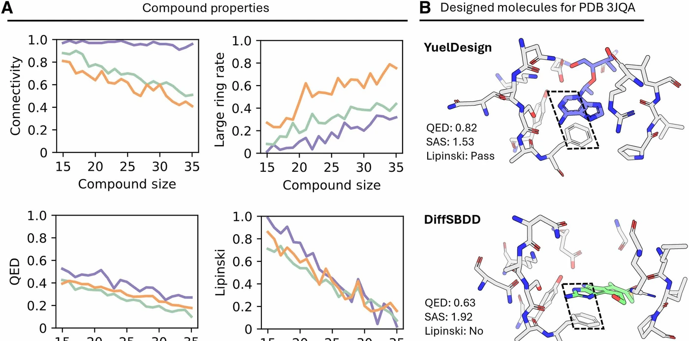
Connectivity asks whether all the atoms ended up in one bonded piece. It is the metric that degrades most obviously with size, because more atoms means more chances for a fragment to drift off, and it is where the gap against DiffSBDD and PMDM is clearest.

Large rings — cycles of more than six atoms — are the other structural failure, hard to synthesise and bad for drug-likeness. YuelDesign produces the fewest across every size range.

A grid of six metrics plotted against compound size: connectivity, macrocycle formation rate, drug-likeness, Lipinski compliance, synthetic accessibility and validity, comparing YuelDesign against DiffSBDD and PMDM.
Figure 2A. Six metrics against compound size, in heavy atoms. YuelDesign, DiffSBDD and PMDM. Drug-likeness declines with size for all three, which is expected — the score penalises molecular weight — and Lipinski compliance falls for the same reason. Synthetic accessibility is close to identical across methods, and validity sits near 1.0 for everyone except PMDM at size 35.

The chemistry it reaches for

The same functional groups, plus a tell.

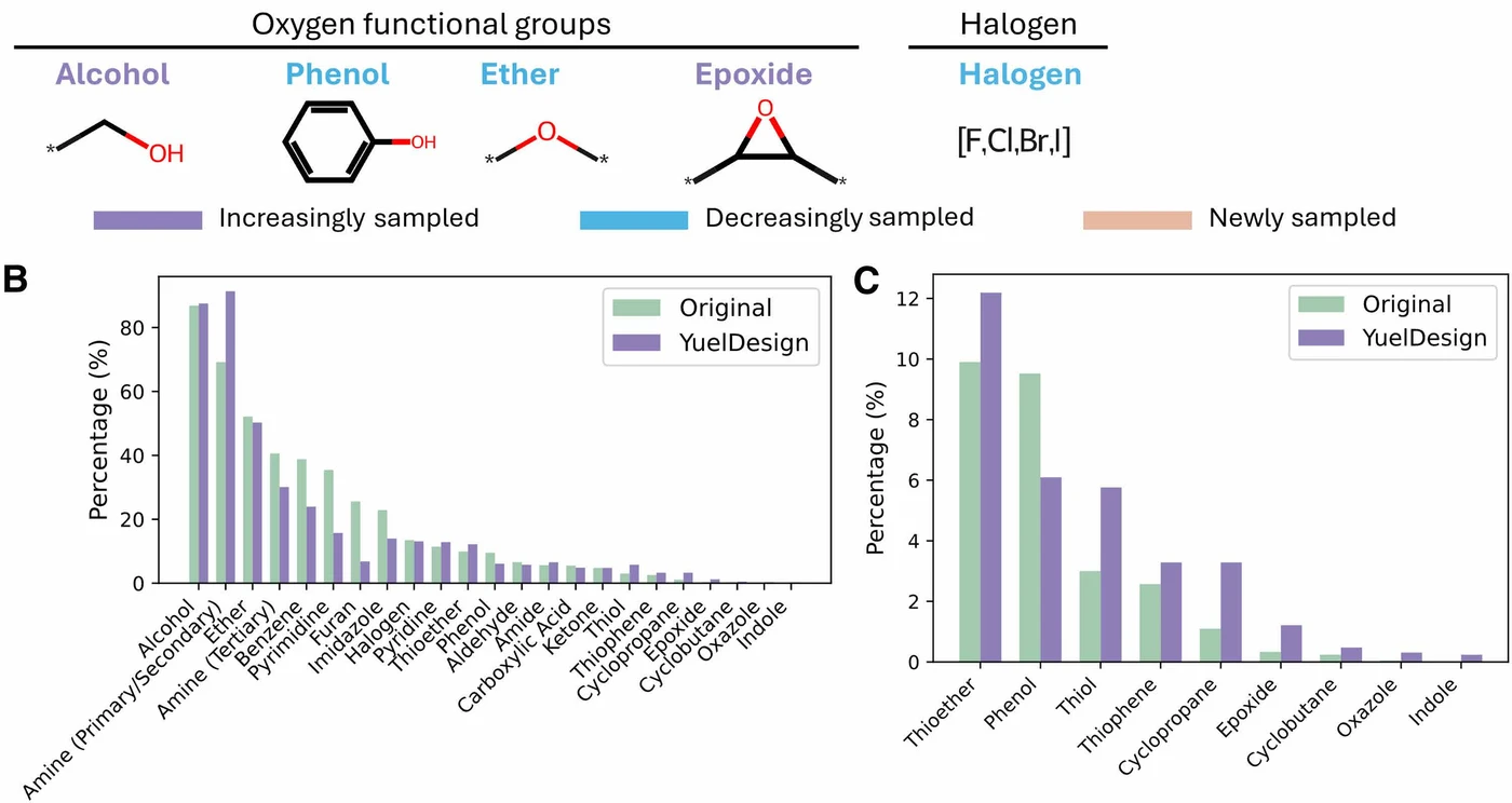
Compared against native ligands, the distribution of functional groups is broadly similar. Alcohols appear in around 85% of molecules in both sets. Amines are in roughly 70% of native ligands and around 90% of generated ones.

The interesting discrepancy is small strained rings — cyclopropane, cyclobutene, epoxide. They are rare in both but enriched in the generated set, and the authors give the mechanism: when you sample atoms from Gaussian noise, three and four-membered rings form easily because they violate no bond length or angle constraint. Nothing in the process knows they are strained.

Bar charts comparing the percentage of molecules containing each functional group, native ligands against YuelDesign output, with a second panel for rarer groups including small strained rings.
Figure 3B, 3C. Native ligands in green, YuelDesign in blue. The first panel covers common groups, the second the rarer ones where the strained-ring enrichment is visible.

Now the pocket itself

How far is a generated pocket allowed to drift?

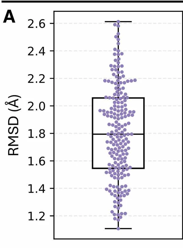
Since the pocket is an output, it can be scored like one. Median deviation from the real structure is 1.8 Å.

Whether that is good depends on a number the paper supplies itself: Brylinski and Skolnick found that across 521 apo-holo pairs, 80% differ by 1 Å or less. So real pockets typically move less than these generated ones do. The paper frames 1.8 Å as reasonable because a much larger value would mean nonsense side chains, which is fair — but a reader should notice that the model is more mobile than the biology, not less.

A box and swarm plot of root mean square deviation between generated pocket structures and their experimental counterparts, centred near 1.8 angstroms.
Figure 4A. Deviation of each generated pocket from its experimental structure. Median 1.8 Å, interquartile range roughly 1.55 to 2.05 Å, whiskers out to about 1.1 and 2.6 Å.

Does the flexibility buy anything measurable

Better docking scores, and poses that survive redocking.

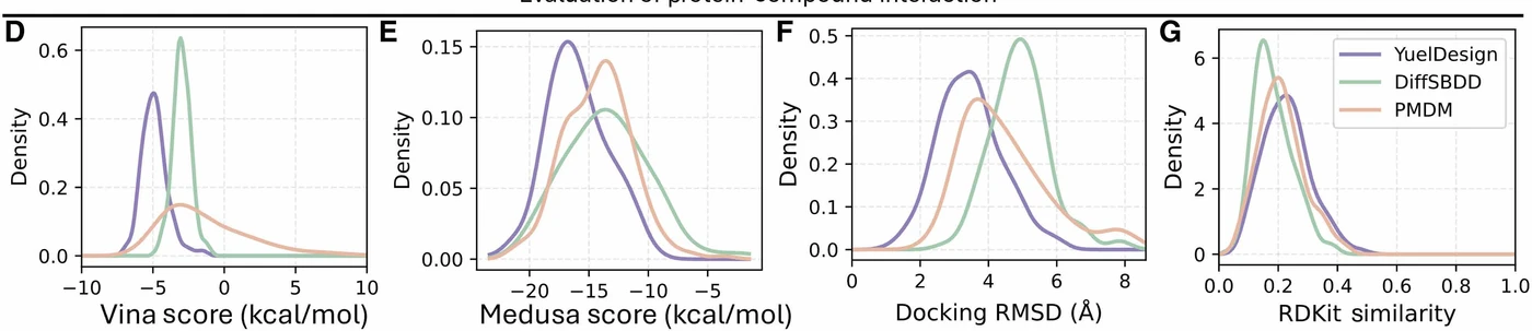
Two scoring functions agree that YuelDesign's molecules bind their pockets better than the rigid baselines' do. More telling is the redocking panel: take the designed molecule, dock it back into the pocket from scratch, and measure how far the new pose lands from the designed one. YuelDesign's poses move least, meaning the geometry it invented is the geometry a docking program independently agrees with.

The similarity panel is the honest counterweight, and it is discussed in the edges section below.

Four density plots: AutoDock Vina score, MedusaDock score, redocking root mean square deviation, and RDKit fingerprint similarity to the native ligand, each comparing the three methods.
Figure 4D–4G. YuelDesign purple, DiffSBDD green, PMDM salmon. For the two score panels more negative is stronger binding, and YuelDesign's distribution sits furthest left in both. In the redocking panel lower is better agreement, and YuelDesign peaks around 3.5 Å against roughly 5 Å for DiffSBDD. The final panel is fingerprint similarity to the native ligand: all three peak between 0.15 and 0.25, which is low for everyone.
05

THE PROOF

One protein, chosen because it cannot be faked

CDK2 has a lock
that has to open.

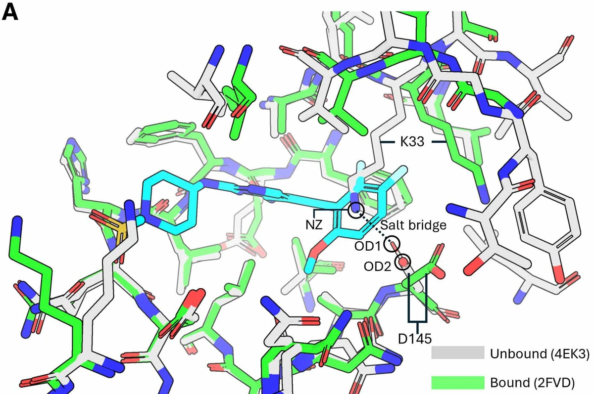
Everything above is a scoreboard. This section is the argument. Cyclin-dependent kinase 2 has a salt bridge in its unbound form between lysine-33 and aspartate-145, measured at 2.84 Å in the bound reference structure. When an inhibitor binds, that bridge breaks and D145 swings to engage the ligand instead.

This makes CDK2 a test that a rigid-pocket method cannot pass by getting lucky. If the pocket is frozen in a conformation where K33 and D145 are bonded to each other, D145 is not available to the ligand. Not unlikely — unavailable.

The conformational switch

The same residues, two states.

Superposing unbound CDK2 on an inhibitor-bound structure shows what has to happen. In the unbound form the lysine nitrogen and the aspartate oxygens are close enough to bond. In the bound form they are not, because the aspartate has moved to make contacts with the inhibitor.

The paper lists four separate CDK2 complexes where D145 interacts favourably with the inhibitor, across four unrelated chemical series. This is not a quirk of one structure.

Unbound CDK2 in grey superposed on the inhibitor-bound structure in green, with the lysine 33 nitrogen and aspartate 145 oxygens labelled and the salt bridge between them marked.
Figure 5A. Unbound CDK2 (4EK3) in grey, inhibitor-bound CDK2 (2FVD) in green, the inhibitor in cyan. The dotted line marks the K33 NZ to D145 OD1 salt bridge present in the unbound state. Compare the grey and green positions of D145 to see the swing.

What each model actually produced

Three molecules, one pocket, one difference.

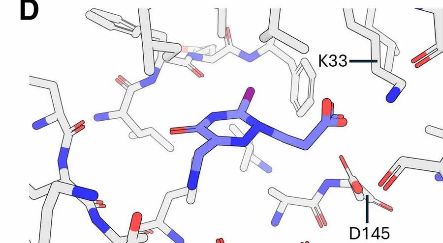
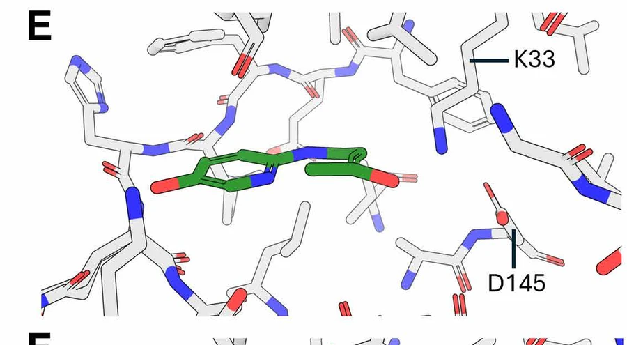
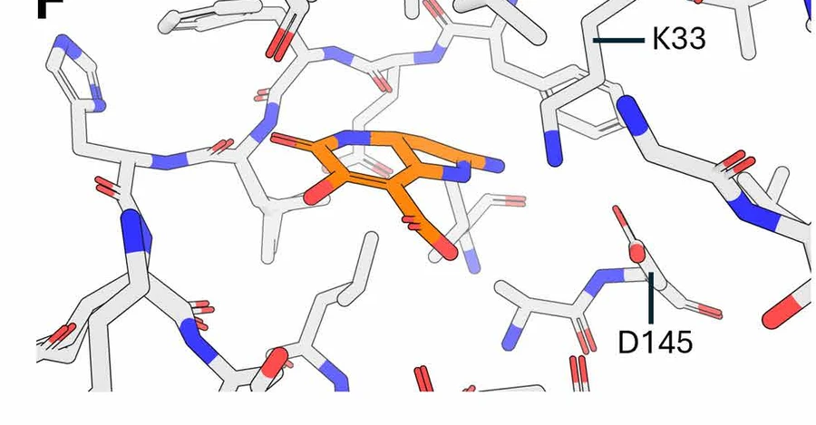
All three methods were asked to design into CDK2. Step through them and watch D145 on the right of each panel. The question is not which molecule looks better — it is whether the molecule is in contact with D145 at all.

The YuelDesign molecule in purple inside the CDK2 pocket, positioned so that it reaches aspartate 145. The DiffSBDD molecule in green inside the same pocket, sitting away from aspartate 145. The PMDM molecule in orange inside the same pocket, also away from aspartate 145.

Counted across every molecule

Twice as many reach the residue.

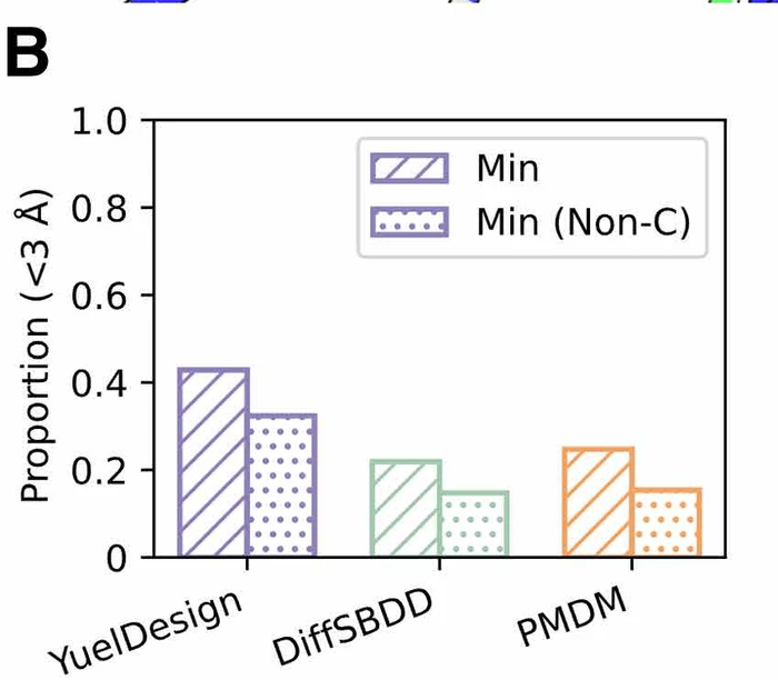
The proportion of generated molecules that come within 3 Å of D145 is roughly 0.43 for YuelDesign against about 0.22 and 0.25 for the two rigid-pocket methods. Restricting to non-carbon atoms, the ones capable of polar or ionic contacts, the numbers are roughly 0.33 against 0.15 and 0.16.

Note that the rigid methods are not at zero. A ligand can approach D145 without the salt bridge breaking. What it cannot do is take the position the native inhibitors take.

Bar chart of the proportion of generated molecules whose minimum distance to aspartate 145 is under three angstroms, for all atoms and for non-carbon atoms only, across the three methods.
Figure 5B. Hatched bars use the minimum distance over all atoms; dotted bars use non-carbon atoms only. Purple YuelDesign, green DiffSBDD, orange PMDM.

The panel that carries the whole paper

Only one method can have a distribution here at all.

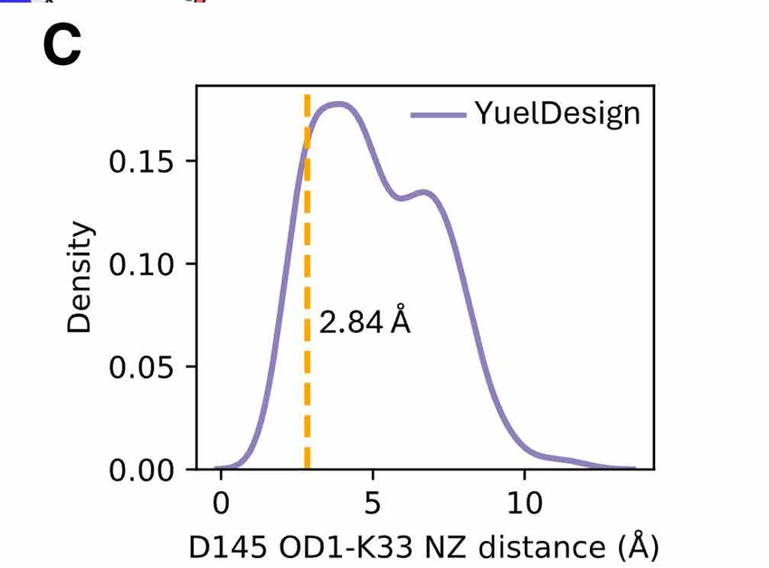
This measures the distance between the two atoms that form the salt bridge, across every generated complex. YuelDesign produces a broad spread from about 2 Å out past 10 Å, including the 2.84 Å of the native bound structure and everything wider.

DiffSBDD and PMDM do not appear on this plot, and that absence is the finding. They hold the pocket fixed, so for them this distance is one number, the same for every molecule they generate. There is no distribution to draw. The salt bridge cannot break because nothing in those models is allowed to move it.

A density curve of the distance between the aspartate 145 and lysine 33 atoms across generated complexes, spanning roughly 2 to 12 angstroms, with the native bound value of 2.84 angstroms marked.
Figure 5C. Distance between D145 OD1 and K33 NZ across YuelDesign's generated complexes. The dashed line marks 2.84 Å, the value in the bound reference structure 2FVD. The curve is bimodal: one population near the native bound geometry, another wider open state around 7 Å.
06

INSIDE

What the process actually does

Shape settles before chemistry does.

The final section of the paper tracks a single generation, step by step, and it is the most useful part for anyone who wants to modify this rather than use it.

One generation, five snapshots

From a cloud to a molecule.

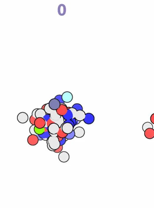
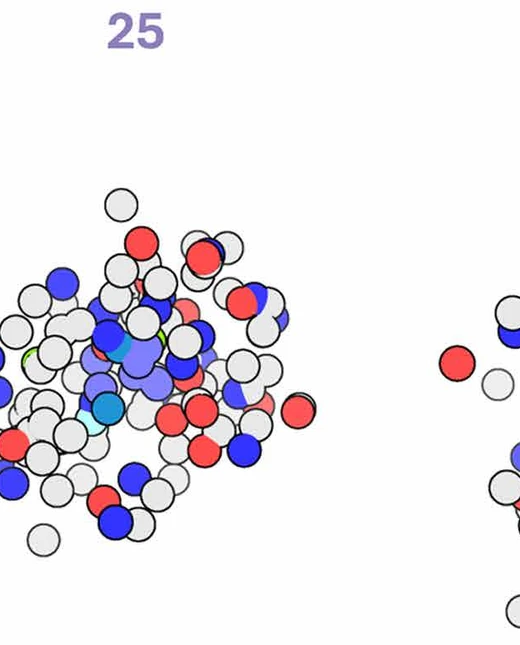
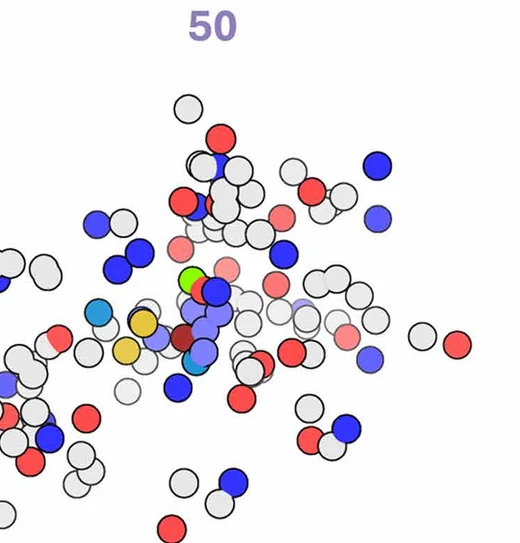
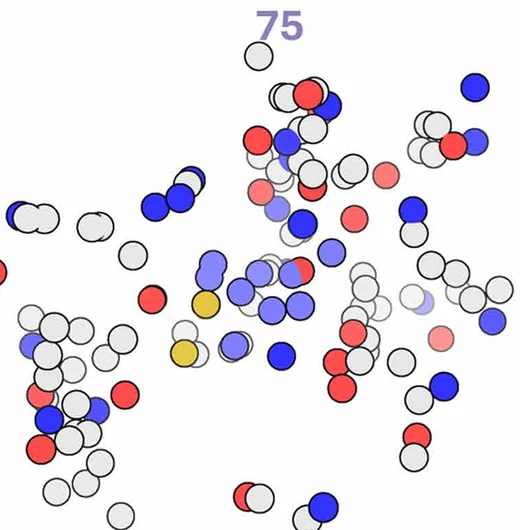
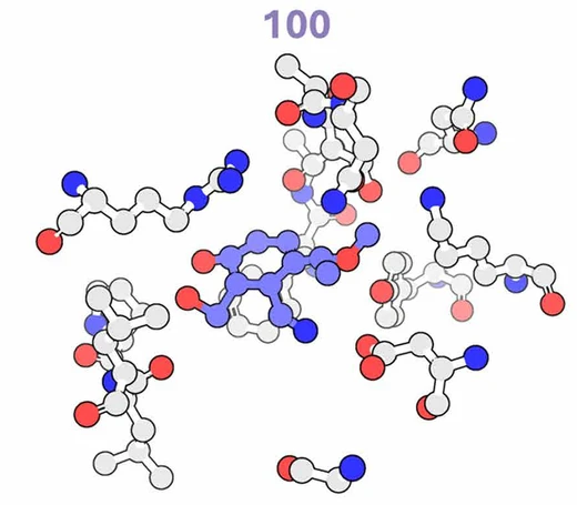
Step through the process. Colours are atom types: grey carbon, blue nitrogen, red oxygen, and the occasional sulfur and phosphorus. At step 0 everything is a tight blob of Gaussian noise with no structure and no meaningful identity.

Diffusion step 0: a tight cluster of coloured spheres with no molecular structure. Diffusion step 25: the atoms have dispersed into a loose cloud with no bonds drawn. Diffusion step 50: atoms spread further apart with local groupings starting to appear. Diffusion step 75: partial bonded fragments are visible among the loose atoms. Diffusion step 100: a fully bonded three-dimensional molecule.

Two clocks, running at different speeds

Positions converge steadily. Bond lengths snap.

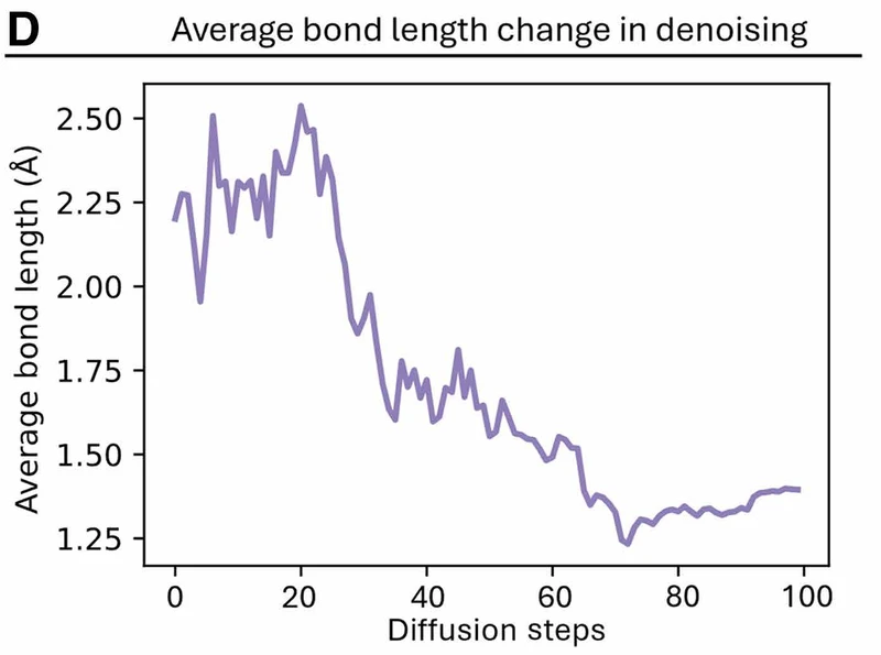
Deviation from the final structure falls smoothly and almost monotonically across the whole run, with no plateau — the coordinates are still tightening at step 90. Average bond length behaves completely differently: it climbs to about 2.5 Å around step 20 as atoms spread out of the initial blob, then falls to roughly 1.35 Å by step 70 and stays there.

That 1.35 Å is a real carbon-carbon single bond. So the moment the molecule becomes chemically plausible is around step 70, well before the coordinates finish settling.

A line plot of average bond length across denoising steps, rising to about 2.5 angstroms near step 20 then falling to roughly 1.35 angstroms by step 70 and flattening.
Figure 6D. Average bond length across the run. The rise to 2.5 Å is atoms dispersing out of the noise blob; the fall to about 1.35 Å is bonds reaching real chemical distances. The flat tail after step 70 is what stabilisation looks like.

And the bonds themselves

Frantic rewiring, then quiet.

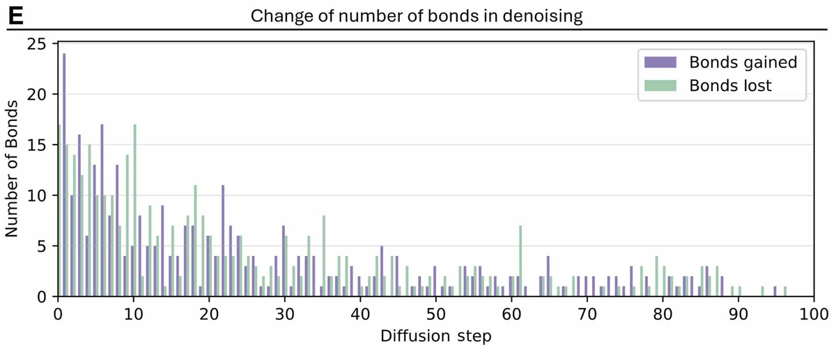
Recomputing bonds at every step from interatomic distances shows around 24 bonds forming and 17 breaking in the first few steps, as atoms pass close to each other in the collapsing cloud. By step 30 the churn is down to a handful per step and it stays low.

Atom identity is the slowest thing to settle. Most type changes happen in the first fifteen steps, but scattered flips continue out to around step 82. Coordinates, bonds and identity therefore finalise in that order, which is why the authors suggest decoupling type determination from coordinate refinement as a possible efficiency gain.

A bar chart of bonds gained and bonds lost at each denoising step, very high for the first ten steps and settling to a few per step after step thirty.
Figure 6E. Bonds gained in purple, bonds lost in green, per step. The early spike is the model sorting out which atoms are neighbours; the long quiet tail is refinement.
07

THE EDGES

Most of these the authors raise themselves

What this does not do.

01

The molecules are not much like the real ones

Fingerprint similarity to the native ligand peaks between 0.15 and 0.25 for all three methods. YuelDesign is marginally higher and the authors say so plainly, attributing it to the size of chemical space. It is worth being clear about what this means: these models are not recovering known binders, they are producing novel molecules whose quality is judged by docking scores rather than by any experiment.

02

Strained rings come free with the noise

Three and four-membered rings are overrepresented because nothing in the sampling process forbids them — they satisfy bond lengths and angles perfectly well while being synthetically awkward and chemically strained. Fixing this needs explicit chemical constraints during generation, which the framework does not have.

03

It degrades on larger molecules

Every atom carries coordinates and a feature vector, and diffusion operates on all of them at once, so dimensionality grows with molecule size. The authors report slower convergence and accumulating error, showing up as worse validity and connectivity at the top of the size range, and propose latent diffusion as the fix. That is a proposal, not a result.

04

The generated pocket moves more than real pockets do

A median deviation of 1.8 Å sits above the 1 Å that 80% of real apo-holo pairs stay within, by the paper's own citation. The flexibility that makes the CDK2 result possible is not free — some of that motion is presumably not biological, and the paper does not separate useful rearrangement from noise.

05

Everything is computational

Vina and MedusaDock are scoring functions, not experiments, and redocking agreement measures self-consistency rather than truth. Nothing here has been synthesised or assayed. That is normal for this literature and it is still the gap between a promising generative model and a drug.

THE SHORT VERSION

The result is not a better molecule.
It is a molecule the others could not reach.

Generate pocket and ligand togetherSide chains rearrange during denoisingInternal contacts can breakNative-like binding modes become available

Most method papers argue on a scoreboard, and this one has a scoreboard: better docking scores, better connectivity, fewer strained macrocycles. But the scoreboard is not the case. The case is one salt bridge in one kinase, and the observation that a rigid-pocket model cannot break it no matter how good its chemistry is. Once you accept that binding sites reorganise, freezing them stops being a simplification and becomes a constraint on what can be designed. The cost is an order of magnitude more atoms to generate, and the paper is honest that this cost is currently what limits it.

READ IT YOURSELF

The paper,
in full.

Published open access under a Creative Commons Attribution 4.0 licence, which is why every figure on this page can be shown here with attribution. Mirrored locally so the download works regardless of what the publisher is doing.

COLOPHON

An interactive reading of Wang, Zhang, Budakoti & Dokholyan, Science Advances 2026. All numbered figures are reproduced from the paper under its CC BY 4.0 licence. Diagrams in the opening sections are drawn for this page and are schematic, not reproductions of data. The work was supported by the National Institutes of Health (1R35 GM134864) and the National Science Foundation (2210963).